More on pressure gradient

Pressure Gradient Breakthrough

I decided to investigate the Cordova-Anchorage pressure gradient a little more given the relatively weak correlation compared to the intuitively strong association, as well as the lag that exists between strong wind events and the time of the maximum gradient.

I realized that the change in the gradient over time might have a better physical connection as it would account for the isallobaric wind. Without pulling any new data, I just used the gradient at the time of the report and the maximum gradient to determine the change over time. I plan on trying to analyze the pressure gradient change centered around or just prior to the wind report next.

The result was a 0.56 correlation to the wind magnitude. This was a notable increase from the maximum gradient correlation. More importantly, when replaced in the empirical formula, it makes a significant difference.

In addition, I have rerun the pressure gradient program to be able to pull data from one event that was missing from the initial database. This is the weakest case, and thus an especially important case.

First of all, it actually reverses the dominant group ... the pressure correlation is 0.61 for the wet class and 0.54 for the dry class. The new correlation for the bestfit values is 0.84 overall, which is excellent ... 0.85 for the wet class, and 0.83 for the dry class. This is a huge improvement. Case-by-case, this also removes the biggest outlier! There are two cases with error greater than 10kt. The average error is 4.4kt or 6.0%

Splitting cases into wet and dry events

Following the information I found from the mid level (3.5km) dew point, I split the cases into wet and dry events, using -30C as a benchmark.

I reanalyzed all of the variables in the empirical formula given the class of the event (wet/dry), for a new average, standard deviation, and correlation to the actual data.

In addition, I added the dew point variable itself into the formula given that especially the dry cases show a strong correlation to the wind magnitude (drier mid levels = stronger winds).

The latest formula incorporates the following variables:

• Cordova-Anchorage SLP gradient
• Depth of the mid-level temperature inversion
• 2.5-5km shear magnitude
• Change in low-level cross-barrier flow over time
• 3km temperature
• 3.5km dew point

The results are very good. Of most significance, the new formula reduces the error of the outliers.

For the wet cases: Correlation = 0.73, Error = 5.0kt, 6.7%

For the dry cases: Correlation = 0.83, Error = 3.9kt, 5.2%

Overall: Correlation = 0.75, Error = 4.6kt, 6.1%

The 0.83 correlation for the dry cases is excellent.

Dew point

Examining the vertical profile of dew point in the Anchorage soundings, there is significantly greater variance than with temperature. The most interesting feature in the composites is between 3000m and 4000m where there is a dry layer in the strong cases and a relatively more moist layer in the weak cases.

I plotted 3500m dew point against the magnitude of the wind event. The huge variance is clear but what stands out the most is that there are two very distinct groups of dew point values. There is a moist group and a dry group. I went ahead and split the data accordingly (color coded on the graph), and analyzed them separately. For both there is a negative correlation between dew point and the wind events ... drier mid levels are conducive to stronger wind events. The correlation is much greater for the dry events (-0.40) then the moist events (-0.22).

Together, there is actually very little correlation between the dew point and wind magnitude, as both the moist and dry classes span a wide spectrum of wind speeds. It's when they're split that we can better identify possible relationships.

This poses the question: Should all events be initially identified as dry or moist before any further analysis be done? Next plan is to redo some of the previous analysis split into these two categories.

Below I have included sounding composites for the dry (red) class and moist (blue) class. These classes also maintain themselves through the 12-24 hour period leading up to the event. So for instance a dry event in this classification maintains a dry profile during the time of the event itself.

Up Next

Whittier to Anchorage pressure gradient

Empirical formula improvement

Investigate physical basis behind 3km temperature correlation

Cross-barrier flow

Cross-barrier flow was one of the parameters I investigated in the individual soundings from each event. As I mentioned here, this parameter exhibited a negative correlation to the wind gust magnitude which goes against intuition. This correlation was largest around 18 to 24 hours prior to the event, and then weakened toward the time of the event at which point it became slightly positive.

From this information, I chose to investigate the change in the cross-barrier flow over time in relation to the wind events. As suggested by the initial statistics, increasing cross-barrier flow correlates with stronger wind events. This at least makes more sense intuitively. The result is a +0.29 correlation. 

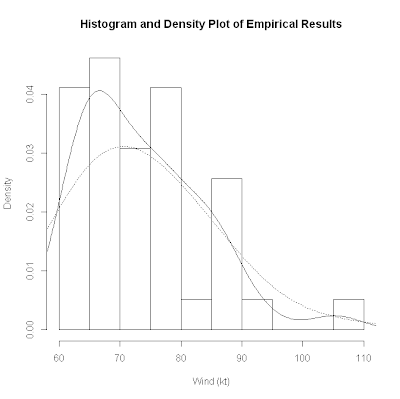
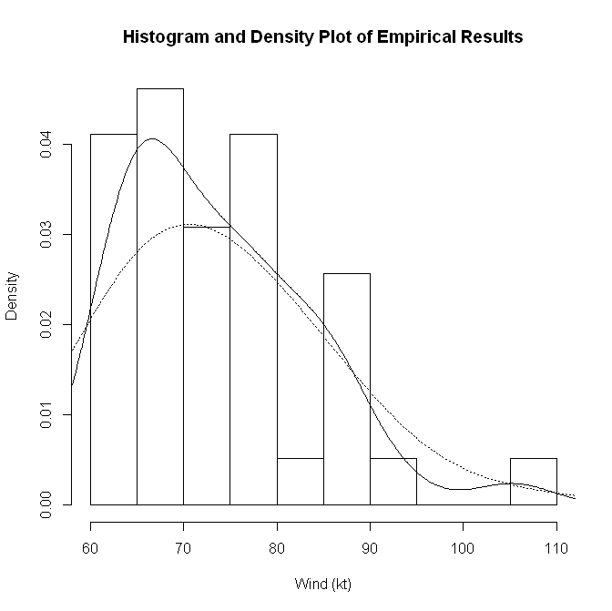
Below I have graphed the wind reports against the d(Cross-barrier flow)/dt parameter. I have included this parameter in the empirical function, which made very slight improvements on the correlation and error. It currently has a correlation of +0.69 with an average error of 4.8kt or 6.5%. The contribution from each component of the function is also plotted. 

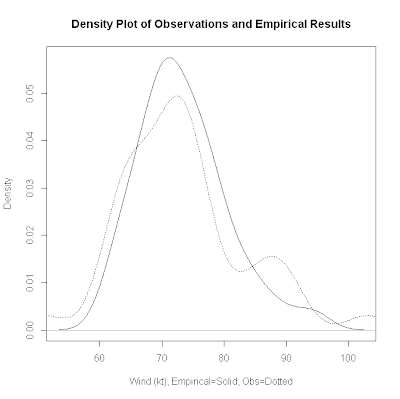
The third graph is the current best fit plot which adjusts for the same standard deviation as the wind event database, and thus it is perfectly averaged around the y=x line on the plot of obs versus empirical values. There are three events for which the empirical value has an error greater than 10kt and eight events with a percent error greater than 10%.

Empirical Formula Formulation

So far I have used the 3000m temperature (correlation = -0.64), the maximum ACV-ANC pressure gradient (+0.40), the depth of the temperature inversion aloft (+0.27), and the 2500-5000m shear (+0.49).

Using these variables weighted by their correlation, I have created an empirical formula with a correlation of +0.68 to the observed winds, and an average error of 4.8kts or 6.5%.