Hodograph composites

The graph below displays the magnitude of vertical wind shear from Z height to 5000m for strong cases (on x-axis) versus weak cases (on y-axis). The greater the distance from the y=x (45deg) line (gray line on graph), the more uniqueness there is between the strong and weak cases. The strong cases exhibit greater vertical wind shear throughout the entire column, but this difference is maximized in the mid levels (can also be seen in the length of the composite hodographs above).

The second graph displays the angle the <strong, weak> vector. The greater the difference from 45 degrees, the more unique the two classes are. We can see that this is maximized at 2500m. More specifically, the 2500m-5000m layer shear exhibits the greatest difference between the strong and weak classes, and thus is the best layer at distinguishing between the two.

Also I created a histogram and density graph of the wind events for future reference in comparing to empirical results:

More on 3000m temperature

As I showed yesterday, there seems to be a strong clustering of the strong case soundings around -16.5C at 3000m, while there is significant spread in the weak cases at this level. I went ahead and pulled temperature data for all 41 cases, and plotted the wind report against the absolute difference from T3000m=-16.5C. The result was a -0.52 correlation ... very impressive for a seemingly arbitrary variable.

From here, I molded this variable to maximize the correlation, and then standardized it to the mean and variance of the actual wind reports. The result was a 0.64 correlation, with an average error of 7.7kts or 10.4%. Again, this is impressive for a single variable, and shows promise for the construction of a useful predictive empirical formula.

First round of various sounding results

So far, the results of spaghetti plot and composite soundings have shown that there is considerable variance in the height and amplitude of pertinent features. Averaging smooths these features down to essentially a constant lapse rate sounding. From the previous tests, the primary inversion layer is generally found near and above 2000m, which can be seen in the spaghetti plot.

To supplement the average, I also plotted the standard deviation of the temperature at each level. This has interesting results. The spread of the weak cases generally increases with height, while the strong cases actually significantly converge around -16.5C at 3000m, at which point the standard deviation drops to near just one degree C. This is around the height that an inversion or stable layer is most likely to be present, and thus the lapse rate is very small or negative.

The plots below are for 18 hours from the time of the event report. Other times are being analyzed now, and show similar results.

Plans for week 3

I have finished the sounding composite program. The averaging tends to smooth much of the detail out of the soundings, so to supplement the composite, I'll include each case sounding overlaid on the same plot. This will give some idea of the spread and common features. I will do this for the top 10 strong cases and bottom 10 weak cases.

Download NARR data for top 5-10 cases and bottom 5-10 cases to initialize WRF. Model should be run 18 hours from the time of event to 6 hours after, each for 24 hours.

From the model data, I am interested in finer time resolution soundings and locations of features that I have pointed out in the synoptic composites.

From this information, combined with the Anchorage-Cordova pressure gradient, and the sounding parameter data, I can construct an empirical predictive formula. I have already ran a few tests that return a greater than .50 correlation and only only a 7% error.

Sounding Parameters

Using a program to pull sounding data from the U Wyoming archive, I was able to isolate certain characteristics of each case sounding. I focused on three primary supporting features of high wind events:

• Low level cross-mountain flow
• Critical level where cross-mountain flow drops to zero
• Inversion or stable layer aloft

To produce quantitative data, I averaged the sfc-850mb wind for cross-mountain flow, yielding an average direction, average speed, and the component crossing the mountain from the southeast. I calculated the height of the critical level by the level at which the component of the wind cross the mountain dropped below 5kt. I tested for the existence of an inversion layer between 850mb and 500mb, and determined the height of the bottom of the inversion as well as the vertical depth of the inversion.

These six variables were then compared to the magnitude of the wind report in each event. The inversion and critical level data was promising: The stronger events more frequently had an inversion present, with the bottom at a lower height than for weak events, and the depth of the inversion larger than for weak events.

The critical level was also generally at a lower height for strong events and higher, or not present at all during weak events.

Interestingly, the cross-mountain flow shows a small negative correlation to the magnitude of the wind event, which I'm not sure what to make of ... weaker events tended to have stronger low level cross-mountain flow...

Quantitative Data

Beginning with the Anchorage-Cordova pressure gradient, I want to look at more quantitative data in order to develop an empirical forecast method. The composite maps give excellent qualitative information on the synoptic situation. One possibility is to pull the prevalent features from the composites to produce usable data. My current project is to examine sounding data, generating quantitative information for each case on the important features (Case Soundings). I have begun writing a program to pull this data from the UWyoming archive.

Anchorage-Cordova Pressure Gradient

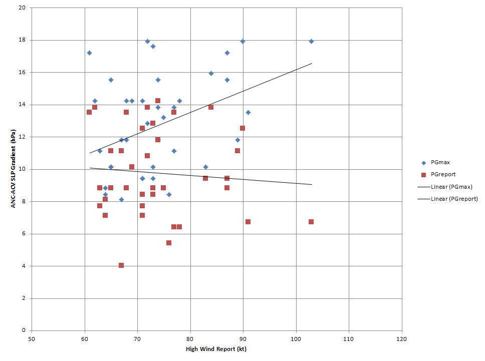
The gradient at the time of the report shows little correlation to the magnitude of the report. The maximum gradient within 18 hours of the report exhibits more of a positive correlation (+0.40).



The time difference shows a positive correlation to the magnitude of the report (+0.31). This suggests that the maximum pressure gradient tends to lead weaker events and lag stronger events.



Possible plan:
Develop an empirical formula for forecasting high wind events.


Important, quantitative factors...